Drum Generation Transformer

Welcome to this partitura tutorial notebook! In this tutorial, we will learn how to train a small auto-regressive transformer model for simplified drum beat generation in MIDI. At the end of this tutorial, we will be able to create a drum beat of a bar’s length and investigate some useful techniques for encoding MIDI as input to a transformer.

Setup

Install packages

If you run it locally, we assume that you cloned the full tutorial repository from https://github.com/CPJKU/partitura_tutorial.git, you are running this notebook from its parent path, and have partitura and the other dependencies installed. Partitura is available in github https://github.com/CPJKU/partitura You can install it with:

pip install partitura

If any other imports fail, please install them in your local environment. If you run it in colab, partitura and other dependencies will be installed automatically.

try:
    import google.colab
    IN_COLAB = True
except:
    IN_COLAB = False

if IN_COLAB:
    !pip install partitura
    !git clone https://github.com/cpjku/partitura_tutorial
    import sys
    sys.path.insert(0, "./partitura_tutorial/notebooks/04_generation/")

Imports

Import the required packages.

%matplotlib inline
import numpy as np
import pandas as pd
import random
import time
import glob
import matplotlib.pyplot as plt
import copy
import pickle
import warnings
warnings.simplefilter("ignore", UserWarning)

import torch
from torch import nn, optim
from torch.utils.data import Dataset, ConcatDataset, DataLoader
from torch.nn import TransformerEncoder, TransformerEncoderLayer
import os
if not IN_COLAB:
    os.environ['KMP_DUPLICATE_LIB_OK']='True'
import partitura as pt

External files

If run locally, external scripts are loaded directly from the cloned tutorial repository.

If run in colab, external scripts are imported by httpimport.

from generation_helpers import (
    INV_PITCH_DICT_SIMPLE,
    tokens_2_notearray,
    save_notearray_2_midifile,
    generate_tokenized_data,
    batch_data,
    PositionalEncoding,
    Transformer,
    sample_from_logits,
    sample_loop
    )

Data Loading

I this tutorial we will work with the groove midi dataset, which contains MIDI drum grooves from a multitude of genres. For simplicity we load only the MIDI files in 4-4 from the dataset. For loading we use Partitura. If you want to load a precomputed and preprocessed dataset you can skip the next cells until the last cell before section 4 where it is loaded.

if IN_COLAB:
    directory = os.path.join("./partitura_tutorial/notebooks/04_generation", "./groove-v1.0.0-midionly")
else:
    directory = os.path.join(os.getcwd(), "./groove-v1.0.0-midionly")

typ_44 = [os.path.basename(f) for f in list(
    glob.glob(directory + "/groove/*/*/*.mid"))
          if "4-4" in f]

beat_type = [g.split("_")[-2] for g  in typ_44]
tempo = [int(g.split("_")[-3]) for g  in typ_44]
vals, counts = np.unique(tempo, return_counts = True)

Histogram of tempos marked in file names

Let’s take a closer look at the data by plotting the histogram of tempi from the target pieces.

plt.plot(vals, counts, c = "r")
plt.hist(np.array(tempo), bins= 60)

(array([  1.,   0.,  10.,  13.,  15.,  18.,  19.,  36.,  42.,  24., 104.,
        110.,  85.,  69.,   8.,  69.,  91., 102.,  82.,  39.,  51.,  16.,
         60.,  42.,  10.,   1.,   0.,   2.,   0.,   0.,   2.,   1.,   3.,
          3.,   0.,   1.,   0.,   1.,   0.,   0.,   0.,   7.,   0.,   0.,
          0.,   0.,   0.,   0.,   0.,   0.,   0.,   0.,   0.,   0.,   0.,
          0.,   0.,   0.,   0.,   1.]),
 array([ 50.,  54.,  58.,  62.,  66.,  70.,  74.,  78.,  82.,  86.,  90.,
         94.,  98., 102., 106., 110., 114., 118., 122., 126., 130., 134.,
        138., 142., 146., 150., 154., 158., 162., 166., 170., 174., 178.,
        182., 186., 190., 194., 198., 202., 206., 210., 214., 218., 222.,
        226., 230., 234., 238., 242., 246., 250., 254., 258., 262., 266.,
        270., 274., 278., 282., 286., 290.]),
 <BarContainer object of 60 artists>)

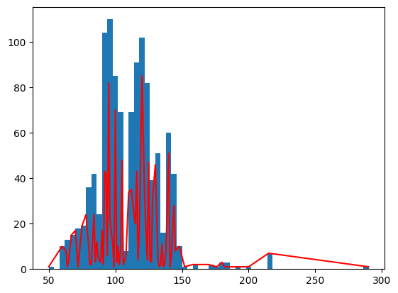
We can almost notice a Gaussian curve with a mean around a 100 beats per minute. Now let’s define the load_data fun

def load_data(
      directory = "./groove-v1.0.0-midionly",
      min_seq_length=10,
      time_sig="4-4",
      beat_type = None
              ):
    """
    loads groove dataset data from directory
    into a list of dictionaries containing the
    note array as well as note sequence metadata.

    Args:
        directory: dir of the dataset
        min_seq_length: minimal sequence length, a
            all shorter performances are discarded
        time_sig: only performances of this time sig
            are loaded
        beat_type: type of beat to load ("beat",
            "fill", or None = both)

    Returns:
        a list of dicts containing note arrays.

    """
    # load data
    files = glob.glob(directory + "/groove/*/*/*.mid")
    files.sort()
    sequences = []
    if beat_type is None:
        beat_types = ["beat", "fill"]
    else:
        beat_types = [beat_type]
    for fn in files:
        bn = os.path.basename(fn)
        bns = bn.split("_")
        tempo = int(bns[-3])
        bt = bns[-2]
        ts = bns[-1].split('.')[-2]
        if ts == time_sig and bt in beat_types:
            seq = pt.load_performance_midi(fn)[0]
            if len(seq.notes) > min_seq_length:
                na = seq.note_array()
                namax = (na['onset_tick'] + na['duration_tick']).max()
                namin = (na['onset_tick']).min()
                dur_in_q = (namax - namin)/seq.ppq
                seq_object = {
                    "id": bn,
                    "na": na,
                    "ppq": seq.ppq,
                    "tempo": tempo,
                    "beat_type": bt,
                    "namax": namax,
                    "namin": namin,
                    "dur_in_q": dur_in_q
                }
                sequences.append(seq_object)
    return sequences

Call the loading function (might take a moment)

seqs = load_data(directory = directory)

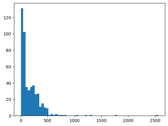
Histogram of performance durations

In this visualization example for the loaded data we plot the histogram of note durations.

dur_in_quarters = [k["dur_in_q"] for k in seqs if k["beat_type"] == "beat"]

plt.hist(dur_in_quarters, bins = 60)
liq = np.array(dur_in_quarters)
print((liq >= 4).sum(), (liq >= -4).sum())

470 484

3. Data Preprocessing: Segmentation & Tokenization

Reducing and Encoding the MIDI Sound Profiles

In this reduces drum generation we encode only 6 main sounds from a list of 22 standard perscussion MIDI sound slots.

Here is a table that shows the Typical Sound to pitch association for drums in MIDI:

MIDI PITCH	STANDARD ASSOCIATED SOUND	REWRITEN SOUND
36	Kick	Kick
37	Snare (X-stick)	Snare
38	Snare (Head)	Snare
40	Snare (Rim)	Snare
43	Tom 1	Tom (Generic)
45	Tom 2	Tom (Generic)
48	Tom 3	Tom (Generic)
47	Tom 2 (Rim)	Tom (Generic)
50	Tom 1 (Rim)	Tom (Generic)
48	Tom 3 (Rim)	Tom (Generic)
48	Hi-Hat Closed (Bow)	Hi-Hat
48	Hi-Hat Closed (Edge)	Hi-Hat
48	Hi-Hat Open (Bow)	Hi-Hat
48	Hi-Hat Open (Edge)	Hi-Hat
49	Crash 1	Crash
55	Crash 1	Crash
52	Crash 2	Crash
57	Crash 2	Crash
51	Ride (bow)	Ride
59	Ride (Edge)	Ride
53	Ride (Bell)	Ride
Any	Default	Default

In summary, we associate all the standard MIDI drum sounds to their sound family, i.e. Snare-type sounds to a Signle Snare sound, and so on.

Reducing the MIDI Velocity Encoding

For MIDI velocity values we encode 8 classes of velocity by applying:

\[newVel = oldVel / 2^4\]

We only accept integer values for \(newVel\), so we are left with 8 classes of velocity.

Reducing the Tempo Encoding

Similarly, we reduce the different tempi found in the training data into 8 classses.

Beat of Fill Characterization

We also add information about each measure of the data being a beat or fill/solo part.

Reducing the Time Encoding

For the time encoding we use a hierarchical tree division in base 2. We start by separating the bar in 2, for first and second half note of the 4/4 bar. We continue for quarter, eight notes, and so on, up to 128 notes. So we use a binary setting for every hierarchical level.

For example the binary hierarchical representation of the second 16th note of the bar would be :

Half Note	Quarter Note	8-th Note	16-th Note	32-th Note	64-th Note	128-th Note
0	0	0	1	0	0	0

PITCH_DICT_SIMPLE = {
    36:0, #Kick
    38:1, #Snare (Head)
    40:1, #Snare (Rim)
    37:1, #Snare X-Stick
    48:2, #Tom 1
    50:2, #Tom 1 (Rim)
    45:2, #Tom 2
    47:2, #Tom 2 (Rim)
    43:2, #Tom 3
    58:2, #Tom 3 (Rim)
    46:3, #HH Open (Bow)
    26:3, #HH Open (Edge)
    42:3, #HH Closed (Bow)
    22:3, #HH Closed (Edge)
    44:3, #HH Pedal
    49:4, #Crash 1
    55:4, #Crash 1
    57:4, #Crash 2
    52:4, #Crash 2
    51:5, #Ride (Bow)
    59:5, #Ride (Edge)
    53:5, #Ride (Bell)
    'default':6
}

def pitch_encoder(pitch, pitch_dict = PITCH_DICT_SIMPLE):
    # 22 different instruments  in dataset, default 23rd class
    a = pitch_dict['default']
    try:
        a = pitch_dict[pitch]
    except:
        print("unknown instrument")
    return a

def time_encoder(time_div, ppq):
    # base 2 encoding of time, starting at half note, ending at 128th
    power_two_classes = list()
    for i in range(7):
        power_two_classes.append(int(time_div // (ppq * (2 **(1-i)))))
        time_div = time_div % (ppq * 2 **(1-i))
    return power_two_classes

def velocity_encoder(vel):
    # 8 classes of velocity
    return vel // 2 ** 4

def tempo_encoder(tmp):
    # 8 classes of tempo between 60 and 180
    return (np.clip(tmp, 60, 179) - 60) // 15

def tokenizer(seq):
    tokens = list()
    na = seq["na"]
    fill_encoding = 0
    if seq["beat_type"] == "fill":
        fill_encoding = 1
    tempo_encoding = tempo_encoder(seq["tempo"])

    for note in na:
        te = time_encoder(note["onset_tick"]%(seq['ppq']*4), seq['ppq'])
        pe = pitch_encoder(note["pitch"])
        ve = velocity_encoder(note["velocity"])

        tokens.append(te + [pe, ve, tempo_encoding, fill_encoding])

    return tokens

def measure_segmentation(seq, beats = 4, minimal_notes = 1):
    mod = beats * seq['ppq']
    no_of_measures = int(seq["namax"] // mod + 1)

    segmented_seq = list()
    for measure_idx in range(no_of_measures):
        na = seq["na"]
        new_na = np.copy(na[na["onset_tick"] // mod == measure_idx])
        if len(new_na) >= minimal_notes:
            new_seq = copy.copy(seq)
            new_seq["na"] = new_na
            segmented_seq.append(new_seq)
        else:
            continue
    return segmented_seq

# try uncommenting the next lines to see the outputs of these functions.
t = tokenizer(seqs[0])
ss = measure_segmentation(seqs[0], minimal_notes = 18)

print("First Tokenized Note of First sequence : {}".format(t[0]))

First Tokenized Note of First sequence : [0, 0, 1, 1, 1, 0, 1, 0, 3, 3, 0]

Training set generation (might take a moment)

train_data = generate_tokenized_data(seqs,
                                     measure_segmentation,
                                     tokenizer,
                                     minimal_notes = 20)
train_dataloader = batch_data(train_data,
                              batch_size=128)

76 batches of size 128

## try uncommenting the next lines to see the outputs of these functions.
# train_dataloader[0].shape # batch, max sequence length, num_tokens

Saving and loading a preprocessed training set

# with open('./dataset129.pyc', 'wb') as fh:
#     pickle.dump(train_dataloader, fh)

# with open('./dataset129.pyc', 'rb') as fh:
#     train_dataloader = pickle.load(fh)

4. Model

The embedding input and output dimension of our model uses the reduced representations that were described above. First, we input with the 7 levels binary hierarchical timing representation in one hot, next instrument (6 classes), velocity (6 classes), tempo (6 classes), and a binary beat as one hot. For the output, every one of those levels also contain a START or END token. Therefore, the binary one-hot representations go from 2 dimensional vectors to 4 dimensional where the third position is for the START token and the fourth position is for the END token.

For consistency we repeated the same dimensions for the input Embeddings of the model. Of course this encodings are up to personal interpretation

class MultiEmbedding(nn.Module):
    '''A Multiembedding'''
    # Initialization
    def __init__(self, tokens2dims):
        super().__init__()
        # self.em_time0 = nn.Embedding(num_tokens, dim_model)
        self.em_time0 = nn.Embedding(tokens2dims[0][0], tokens2dims[0][1])
        self.em_time1 = nn.Embedding(tokens2dims[1][0], tokens2dims[1][1])
        self.em_time2 = nn.Embedding(tokens2dims[2][0], tokens2dims[2][1])
        self.em_time3 = nn.Embedding(tokens2dims[3][0], tokens2dims[3][1])
        self.em_time4 = nn.Embedding(tokens2dims[4][0], tokens2dims[4][1])
        self.em_time5 = nn.Embedding(tokens2dims[5][0], tokens2dims[5][1])
        self.em_time6 = nn.Embedding(tokens2dims[6][0], tokens2dims[6][1])
        self.em_pitch = nn.Embedding(tokens2dims[7][0], tokens2dims[7][1])
        self.em_velocity = nn.Embedding(tokens2dims[8][0], tokens2dims[8][1])
        self.em_tempo = nn.Embedding(tokens2dims[9][0], tokens2dims[9][1])
        self.em_beat = nn.Embedding(tokens2dims[10][0], tokens2dims[10][1])
        # self.total_dim = np.array([[2,2,2,2,2,2,2, # time encoding
        #                  2,2,2,2]]).sum() # instrument, velocity, tempo, beat/fill
    def forward(self, x):
        '''Update Function and predict function of the model'''

        output = torch.cat((
        self.em_time0(x[:,:,0]),
        self.em_time1(x[:,:,1]),
        self.em_time2(x[:,:,2]),
        self.em_time3(x[:,:,3]),
        self.em_time4(x[:,:,4]),
        self.em_time5(x[:,:,5]),
        self.em_time6(x[:,:,6]),
        self.em_pitch(x[:,:,7]),
        self.em_velocity(x[:,:,8]),
        self.em_tempo(x[:,:,9]),
        self.em_beat(x[:,:,10])),
        dim=-1)
        return output

5. Training

def train_loop(model, opt, loss_fn, dataloader, tokens2dims):
    """
    """
    t2d = np.array(tokens2dims)
    pred_dims = np.concatenate(([0],np.cumsum(t2d[:,0])))
    model.train()
    total_loss = 0

    for batch in dataloader:
        y = batch
        y = torch.tensor(y).to(device)

        # Now we shift the tgt by one so with the <SOS> we predict the token at pos 1
        y_input = y[:,:-1,:]
        y_expected = y[:,1:,:]

        # Get mask to mask out the next words
        sequence_length = y_input.size(1)
        tgt_mask = model.get_tgt_mask(sequence_length).to(device)

        # Standard training except we pass in y_input and tgt_mask
        pred = model(y_input, tgt_mask)

        # Permute pred to have batch size first again, that is batch / logits / sequence
        pred = pred.permute(1, 2, 0)
        loss = 0
        for k in range(11):
            # batch / logits / sequence ----- batch / sequence / tokens
            loss += loss_fn(pred[:,pred_dims[k]:pred_dims[k+1],:], y_expected[:,:,k])

        opt.zero_grad()
        loss.backward()
        opt.step()

        total_loss += loss.detach().item()

    return total_loss / len(dataloader)

def fit(model, opt, loss_fn, train_dataloader, t2d, epochs):
    """
    """
    train_loss_list = []

    print("Training and validating model")
    for epoch in range(epochs):
        print("-"*25, f"Epoch {epoch + 1}","-"*25)

        train_loss = train_loop(model, opt, loss_fn, train_dataloader, t2d)
        train_loss_list += [train_loss]



        print(f"Training loss: {train_loss:.4f}")
        print()

    return train_loss_list

Initialize Model

The model figure above sets a clear direction for the input and output dimension of the model. So now we just need to initialize it likewise. The core model we use is a basic Transformer, that is already implemented in Pytorch. The Transformer model is not the focus of this tutorial so therefore we load it from a helper file.

tokens2dims = [
            (4, 8),
            (4, 8),
            (4, 8),
            (4, 4),
            (4, 4),
            (4, 4),
            (4, 4),
            (8, 16),
            (10, 12),
            (10, 12),
            (4, 4)
        ]

model_spec = dict(
    tokens2dims=tokens2dims,
    num_heads=6,
    num_decoder_layers=6,
    dropout_p=0.1
)

device = "cuda" if torch.cuda.is_available() else "cpu"
model = Transformer(
    tokens2dims = model_spec["tokens2dims"],
    MultiEmbedding = MultiEmbedding,
    num_heads = model_spec["num_heads"],
    num_decoder_layers = model_spec["num_decoder_layers"],
    dropout_p = model_spec["dropout_p"],
).to(device)

opt = torch.optim.Adam(model.parameters(), lr=0.002)
loss_fn = nn.CrossEntropyLoss()

pytorch_total_params = sum(p.numel() for p in model.parameters() if p.requires_grad)
print("Number of parameters in model: ", pytorch_total_params)

Number of parameters in model:  264700

6. LOOP (only call to retrain / finetrain)

"""
EPOCH = 1
PATH = "modelname.pt"
LOSS = train_loss_list[-1]
MODEL_SPEC = model_spec

torch.save({
            'epoch': EPOCH,
           'model_state_dict': model.state_dict(),
            'optimizer_state_dict': opt.state_dict(),
            'loss': LOSS,
            'model_spec': MODEL_SPEC,
            }, PATH)
"""

'\nEPOCH = 1\nPATH = "modelname.pt"\nLOSS = train_loss_list[-1]\nMODEL_SPEC = model_spec\n\ntorch.save({\n            \'epoch\': EPOCH,\n           \'model_state_dict\': model.state_dict(),\n            \'optimizer_state_dict\': opt.state_dict(),\n            \'loss\': LOSS,\n            \'model_spec\': MODEL_SPEC,\n            }, PATH)\n'

if IN_COLAB:
    PATH = os.path.join("partitura_tutorial/notebooks/04_generation", "Drum_Transformer_Checkpoint.pt")
else:
    PATH = "Drum_Transformer_Checkpoint.pt"

checkpoint = torch.load(PATH, map_location=torch.device(device))
model.load_state_dict(checkpoint['model_state_dict'])
opt.load_state_dict(checkpoint['optimizer_state_dict'])

train_loss_list = fit(model, opt, loss_fn, train_dataloader, tokens2dims, 1)

Training and validating model
------------------------- Epoch 1 -------------------------
Training loss: 3.6172

7. SAMPLING

To generate a drum beat we need to call sample_loop from the model. The sampling loop will start with a START token in all fields (Timing, tempo, etc.) and autoregressively predict one note at the time until having a pre-specified number of notes.

X = sample_loop(model, tokens2dims, device)

df = pd.DataFrame(X.cpu().numpy()[0,1:,:],
                  columns=['Time Half Note',
                           'Time Quarter Note',
                           'Time 8th Note',
                           'Time 16th Note',
                           'Time 32nd Note',
                           'Time 64th Note',
                           'Time 128th Note',
                           'Pitch / Instrument',
                           'Velocity',
                           'Tempo',
                           'Beat type'])
df

	Time Half Note	Time Quarter Note	Time 8th Note	Time 16th Note	Time 32nd Note	Time 64th Note	Time 128th Note	Pitch / Instrument	Velocity	Tempo	Beat type
0	0	0	0	1	0	0	0	1	4	3	0
1	0	0	0	1	0	1	1	0	5	3	0
2	0	0	0	1	0	1	0	3	4	3	0
3	0	0	0	1	0	0	1	1	6	3	0
4	0	0	0	1	0	1	1	3	5	3	0
5	1	0	0	1	1	1	1	1	7	3	0
6	1	0	1	0	0	1	0	0	5	3	0
7	1	1	1	1	0	0	0	1	4	3	0
8	1	1	1	1	1	1	1	0	4	3	0
9	1	1	1	1	1	1	1	1	7	3	0
10	3	3	3	3	3	3	3	7	9	9	3
11	3	3	3	3	3	3	3	7	9	9	3
12	3	3	3	3	3	3	3	7	9	9	3
13	3	3	3	3	3	3	3	7	9	9	3
14	3	3	3	3	3	3	3	7	9	9	3
15	3	3	3	3	3	3	3	7	9	9	3
16	3	3	3	3	3	3	3	7	9	9	3
17	3	3	3	3	3	3	3	7	9	9	3
18	3	3	3	3	3	3	3	7	9	9	3
19	3	3	3	3	3	3	3	7	9	9	3
20	3	3	3	3	3	3	3	7	9	9	3
21	3	3	3	3	3	3	3	7	9	9	3
22	3	3	3	3	3	3	3	7	9	9	3
23	3	3	3	3	3	3	3	7	9	9	3
24	3	3	3	3	3	3	3	7	9	9	3
25	3	3	3	3	3	3	3	7	9	9	3
26	3	3	3	3	3	3	3	7	9	9	3
27	3	3	3	3	3	3	3	7	9	9	3
28	3	3	3	3	3	3	3	7	9	9	3
29	3	3	3	3	3	3	3	7	9	9	3
30	3	3	3	3	3	3	3	7	9	9	3

We can see that the sample loop predicts 30 notes (apart from the START token) but only 16 actual MIDI notes where predicted and from line 16 and down we get only the END token.

Finally, we can save generated MIDI files from the sampling process.

for k in range(16):
    XX = X.cpu().numpy()[k,1:,:]
    na = tokens_2_notearray(XX)
    save_notearray_2_midifile(na, k, fn = "PartituraTutorialBeats")

Conclusion

This is the end of the Tutorial for drum beat generation using partitura.

To play the MIDI files you can import them in your DAW of preference and load a drum VSTi or create your own DrumSampler.

In this tutorial, we learned how to create MIDI drum generation using partitura and a Transformer autoregressive model. We investigated some possibilities for encoding and tokenization of timing, instrument, dynamics, and tempo.